Determine Dimensionality

Next, we determine dimensionality (how many components to include) using the PCA results.

The top principal components represent a robust compression of the dataset.

A JackStraw procedure-inspired resampling test can be used: randomly permute a subset of the data (1% by default), rerun PCA to construct a “null distribution” of feature scores, repeat the procedure, and identify “significant” PCs as those who have a strong enrichment of low p-value features. This approach is computationally intense.

Alternatively, use an elbow plot, which ranks PCs based on percentage of variance explained by each one. This is much less computationally intense.

JackStraw Test

The JackStraw test randomly permutes a subset of data, and calculates projected PCA scores for these “random” genes. Then, it compares the PCA scores for the “random” genes with the observed PCA scores to determine statistical significance. The end result is a p-value for each gene’s association with each principal component.

pbmc <- JackStraw(pbmc, num.replicate = 100)
pbmc <- ScoreJackStraw(pbmc, dims = 1:20)
JackStrawPlot(pbmc, dims = 1:15)

Output:

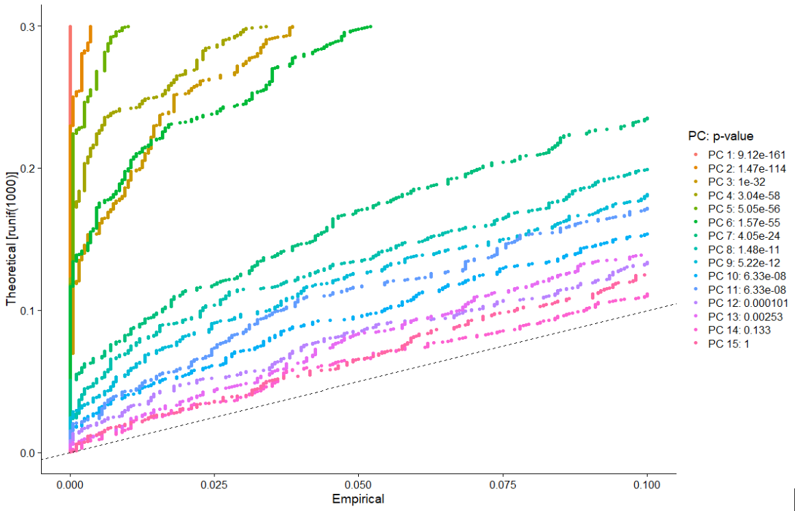
The plot provides a visualization of the statistical test that calculates the significance of your principal components.

Compare the distribution of p-values for each PC with a uniform distribution (represented by the dashed line). “Significant” PCs show a strong enrichment of features with low p-values (curve above the dashed line).

The graph shows a drop-off in significance after the first 10-12 PCs.

Elbow Plot

ElbowPlot(pbmc)

Output:

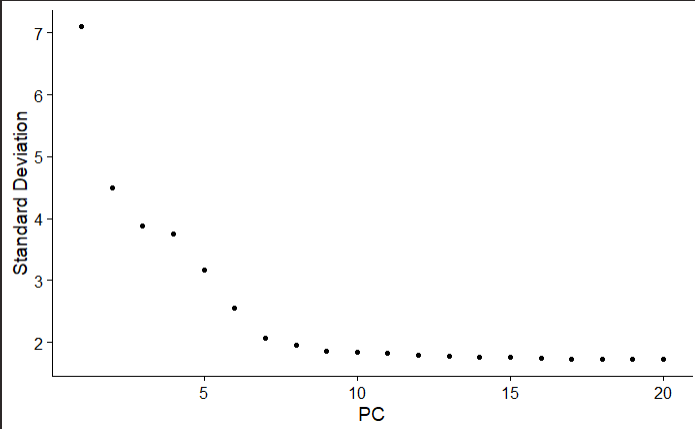
This shows a ranking of principle components based on the percentage of variance explained by each one

Observe an ‘elbow’ around PC 9-10, suggesting that the majority of true signal is captured in the first 10 PCs.

This ‘elbow’ starts at ~PC 7, and definitely flattens off by PC 10, so we will choose PC10 as our cutoff for significant PCs.